How to Read a Grain Size Distribution Graph

Understanding and Interpreting Particle Size Distribution Calculations
Performing a particle size analysis is the best way to respond the question: What size are those particles? Once the assay is complete the user has a variety of approaches for reporting the outcome. Some people prefer a single number answer—what is the average size? More than experienced particle scientists cringe when they hear this question, knowing that a single number cannot describe the distribution of the sample. A better approach is to written report both a central point of the distribution along with i or more values to describe the width of distribution. Other approaches are also described in this web page.
Central Values: Mean, Median, and Way
For symmetric distributions such as the i shown in Figure 1 all central values are equivalent: mean = median = mode. But what do these values represent?
Mean

Mean is a calculated value similar to the concept of average. The diverse mean calculations are divers in several standard documents (ref.1,ii). In that location are multiple definitions for mean because the mean value is associated with the basis of the distribution adding (number, surface, volume). See (ref. 3) for an caption of number, surface, and volume distributions. Laser diffraction results are reported on a volume basis, so the book mean can exist used to define the cardinal point although the median is more than frequently used than the hateful when using this technique. The equation for defining the volume mean is shown below. The best way to call back most this calculation is to retrieve of a histogram table showing the upper and lower limits of n size channels along with the percent within this aqueduct. The Di value for each channel is the geometric mean, the square root of upper ten lower diameters. For the numerator take the geometric Di to the fourth ability multiplied by the percent in that channel, summed over all channels. For the denominator accept the geometric Di to the third power multiplied past the percentage in that aqueduct, summed over all channels. 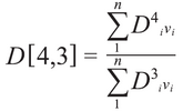
The volume mean diameter has several names including D4,3. In all HORIBA diffraction software this is simply chosen the "hateful" whenever the result is displayed as a volume distribution. Conversely, when the result in HORIBA software is converted to a surface area distribution the mean value displayed is the surface mean, or D3,2. The equation for the surface hateful is shown beneath. 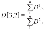
The description for this calculation is the aforementioned as the D4,3 calculation, except that Di values are raised to the exponent values of 3 and 2 instead of 4 and three. The generalized form of the equations seen above for D4,three and D3,2 is shown beneath (post-obit the conventions from ref. 2, ASTM Due east 799). 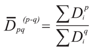
Where:
Some of the more mutual representative diameters are:
The case results shown in ASTM E 799 are based on a distribution of liquid droplets (particles) ranging from 240 - 6532 µm. For this distribution the following results were calculated:
These results are adequately typical in that the D(iv,3) is larger than the D50 - the volume-ground median value.
Median
Median values are divers equally the value where one-half of the population resides above this point, and one-half resides below this point. For particle size distributions the median is called the D50 (or x50 when post-obit certain ISO guidelines). The D50 is the size in microns that splits the distribution with half above and half beneath this bore. The Dv50 (or Dv0.5) is the median for a book distribution, Dn50 is used for number distributions, and Ds50 is used for surface distributions. Since the primary effect from laser diffraction is a book distribution, the default D50 cited is the volume median and D50 typically refers to the Dv50 without including the v. This value is one of the easier statistics to understand and besides one of the about meaningful for particle size distributions.
Mode

The mode is the elevation of the frequency distribution, or it may exist easier to visualize it every bit the highest peak seen in the distribution. The mode represents the particle size (or size range) most commonly found in the distribution. Less care is taken to denote whether the value is based on volume, surface or number, so either run the risk of assuming volume basis or check to clinch the distribution ground. The manner is not as commonly used, but can be descriptive; in detail if at that place is more than one peak to the distribution, then the modes are helpful to describe the mid-indicate of the different peaks. For non-symmetric distributions the mean, median and way volition exist three unlike values shown in Figure ii.
Distribution Widths

Well-nigh instruments are used to measure the particle size distribution, implying an interest in the width or breadth of the distribution. Experienced scientists typically shun using a single number answer to the question "What size are those particles?", and prefer to include a fashion to define the width. The field of statistics provides several calculations to depict the width of distributions, and these calculations are sometimes used in the field of particle characterization. The virtually common calculations are standard difference and variance. The standard departure (St Dev.) is the preferred value in our field of study. Every bit shown in Figure iii, 68.27% of the total population lies within +/- 1 St Dev, and 95.45% lies within +/- 2 St Dev. Although occasionally cited, the use of standard divergence declined when hardware and software advanced beyond bold normal or Rosin-Rammler distributions. One time "model independent" algorithms were introduced many particle scientists began using different calculations to describe distribution width. 1 of the common values used for laser diffraction results is the bridge, with the strict definition shown in the equation below (2): 

In rare situations the bridge equation may be defined using other values such as Dv0.eight and Dv0.2. Laser diffraction instruments should allow users this flexibility. An boosted approach to describing distribution width is to normalize the standard divergence through division by the hateful. This is the Coefficient of Variation (COV) (although information technology may also be referred to equally the relative standard departure, or RSD). Although included in HORIBA laser diffraction software this value is seldom used every bit often as information technology should given its stature. The COV calculation is both used and encouraged as a adding to express measurement event reproducibility. ISO 13320 (ref. 4) encourages all users to mensurate whatever sample at least 3 times, calculate the mean, st dev, and COV (st dev/mean), and the standard sets laissez passer/fail criteria based on the COV values. Another common approach to define the distribution width is to cite three values on the x-axis, the D10, D50, and D90 as shown in Figure 4. The D50, the median, has been divers above as the diameter where half of the population lies below this value. Similarly, 90 percentage of the distribution lies below the D90, and 10 per centum of the population lies below the D10.
Technique Dependence
HORIBA Scientific offers particle label tools based on several principles including laser diffraction, dynamic light handful, and image analysis. Each of these techniques generates results in both like and unique ways. Most techniques can describe results using standard statistical calculations such as the hateful and standard deviation. Only ordinarily accepted practices for describing results take evolved for each technique.
Laser Diffraction
All of the calculations described in this certificate are generated past the HORIBA laser diffraction software package. Results can exist displayed on a volume, expanse, or number basis. Statistical calculations such as standard deviation and variance are available in either arithmetic or geometric forms. The about common approach for expressing laser diffraction results is to report the D10, D50, and D90 values based on a volume distribution. The span calculation is the nearly common format to express distribution width. That said, there is naught incorrect with using any of the available calculations, and indeed many customers include the D4,3 when reporting results. A word of circumspection is given when considering converting a book distribution into either a surface surface area or number footing. Although the conversion is supplied in the software, it is only provided for comparison to other techniques, such as microscopy, which inherently measure out particles on different bases. The conversion is only valid for symmetric distributions and should not be used for any other purpose than comparison to some other technique.
Dynamic Calorie-free Scattering
Dynamic Light Scattering (DLS) is unique amidst the techniques described in this document. The master result from DLS is typically the intensity based harmonic mean value and is typically called the Z-boilerplate. (Encounter the What is the Z-Average? web page for more information). Distribution width is described using the polydispersity index (PDI). It is possible to catechumen from an intensity to a volume or number distribution in order to compare to other techniques.
Paradigm Analysis
The master results from epitome analysis are based on number distributions. These are often converted to a volume ground, and in this case this is an accepted and valid conversion. Image analysis provides far more data values and options than any of the other techniques described in this certificate. Measuring each particle allows the user unmatched flexibility for calculating and reporting particle size results. Image assay instruments may report distributions based on particle length as opposed to spherical equivalency, and they may build volume distributions based on shapes other than spheres. Image analysis tools allow users to choose a variety of length and width descriptors such as the maximum Feret bore and the minimum largest chord diameter as described in ISO 13322-two (ref. five). With the ability to mensurate particles in any number of means comes the decision to report those measurements in any number of ways. Users are over again cautioned against reporting a single value—the number mean existence the worst selection of the possible options. Experienced particle scientists often report D10, D50, and D90, or include standard departure or bridge calculations when using paradigm analysis tools.
Conclusions
All particle size analysis instruments provide the ability to measure and report the particle size distribution of the sample. There are very few applications where a single value is appropriate and representative. The modern particle scientist often chooses to describe the unabridged size distribution as opposed to but a single point on it. (One exception might be extremely narrow distributions such as latex size standards where the width is negligible.) Almost all real globe samples be as a distribution of particle sizes and it is recommended to report the width of the distribution for any sample analyzed. The most appropriate choice for expressing width is dependent on the technique used. When in dubiety, it is often wise to refer to industry accepted standards such as ISO or ASTM in order to arrange to common practice.
References
Technical Notes
Browse Products


PSA300* Static Prototype Assay System Particle Size

Request for Information
Do you accept whatever questions or requests? Use this form to contact our specialists.
Source: https://www.horiba.com/int/static-light-scattering-sls-particle-size-distribution-calculations/
0 Response to "How to Read a Grain Size Distribution Graph"
Post a Comment